Graphs of Inverse Trigonometric Functions Explained – Class 12 Maths

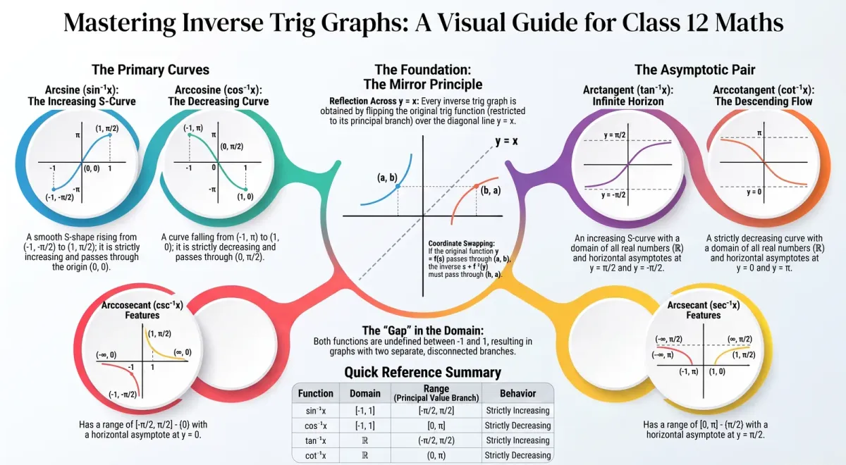
Understanding the graphs of inverse trigonometric functions is more than a visual exercise — it reinforces the concepts of domain, range, and principal value branches in a way that pure algebra cannot. Once you see the graph of y = sin⁻¹ x alongside y = sin x, the relationship between the two becomes immediately clear. This guide walks you through how all six inverse trig graphs are obtained, what they look like, and what properties you can read directly from the graph.

The Mirror Principle: How Every Inverse Trig Graph Is Obtained

There is one fundamental rule that generates all six inverse trig graphs from the original trig graphs: the graph of an inverse function is the reflection of the original function’s graph across the line y = x.

This follows directly from the definition. If y = f(x) passes through the point (a, b), then x = f⁻¹(y) passes through (b, a). Swapping the coordinates of every point on the graph of f gives you the graph of f⁻¹. Geometrically, this is equivalent to reflecting across the diagonal line y = x.

This means: to get the graph of y = sin⁻¹ x from the graph of y = sin x, simply flip the entire picture across y = x. What was on the x-axis becomes the y-axis, and vice versa.

Graph of y = sin⁻¹ x

How It Is Obtained

The graph of y = sin x is a familiar wave extending across all real numbers with range [−1, 1]. When restricted to the interval [−π/2, π/2] — the principal value branch — this portion of the sine curve is a smooth S-shape rising from (−π/2, −1) to (π/2, 1).

Reflecting this restricted portion across y = x gives the graph of y = sin⁻¹ x.

Key Features

• Domain: [−1, 1] — the graph exists only for x between −1 and 1

• Range: [−π/2, π/2] — the graph stretches vertically between −π/2 and π/2

• Shape: S-curve, similar to the arctangent but with finite endpoints

• Endpoints: The graph touches (−1, −π/2) and (1, π/2) — both are included

• Passes through: (0, 0)

• Increasing: The graph is strictly increasing throughout its domain

The dark portion of the sine wave in the NCERT textbook’s Fig 2.1(ii) corresponds to the principal branch — and it is precisely this portion that, when reflected, gives y = sin⁻¹ x.

Graph of y = cos⁻¹ x

How It Is Obtained

The cosine function restricted to [0, π] is strictly decreasing, falling from (0, 1) to (π, −1). Reflecting this arc across y = x gives the graph of y = cos⁻¹ x.

Key Features

• Domain: [−1, 1]

• Range: [0, π]

• Shape: Decreasing curve (top-left to bottom-right)

• Endpoints: (−1, π) and (1, 0)

• Passes through: (0, π/2)

• Decreasing: cos⁻¹ x is strictly decreasing — as x increases from −1 to 1, cos⁻¹ x decreases from π to 0.

This is the key contrast with sin⁻¹ x: arcsine is increasing, arccosine is decreasing.

Graph of y = tan⁻¹ x

How It Is Obtained

The tangent function restricted to (−π/2, π/2) produces all real values, sweeping from −∞ to +∞. Reflecting this across y = x gives a curve that accepts all real inputs but produces outputs only in (−π/2, π/2).

Key Features

• Domain: ℝ — the graph extends infinitely in both horizontal directions

• Range: (−π/2, π/2) — the graph is always strictly between the horizontal asymptotes y = −π/2 and y = π/2

• Shape: Classic S-curve

• Asymptotes: Horizontal lines at y = π/2 (above) and y = −π/2 (below)

• Passes through: (0, 0)

• Increasing: Strictly increasing for all x ∈ ℝ

The horizontal asymptotes are the most distinctive feature of this graph. They reflect the fact that no finite input to tan⁻¹ ever produces the values ±π/2.

Graph of y = cot⁻¹ x

Key Features

• Domain: ℝ

• Range: (0, π)

• Asymptotes: y = 0 and y = π

• Decreasing: Strictly decreasing — cot⁻¹ x falls as x increases

• Passes through: (0, π/2)

Unlike tan⁻¹ x, the graph of cot⁻¹ x falls from top to bottom across the real line, approaching π/2 at x = 0 and descending toward 0 as x → +∞.

Graphs of y = cosec⁻¹ x and y = sec⁻¹ x

Both functions share the same domain — ℝ − (−1, 1) — producing two-branched graphs with a visible gap between −1 and 1.

cosec⁻¹ x: Range [−π/2, π/2] − {0}, with horizontal asymptote y = 0. For x ≥ 1 the branch sits in the first quadrant; for x ≤ −1 it occupies the third quadrant.

sec⁻¹ x: Range [0, π] − {π/2}, with horizontal asymptote y = π/2. For x ≥ 1 the graph increases from (1, 0) toward π/2; for x ≤ −1 it continues upward from π/2 toward π at x = −1.

Reading Properties from the Graphs

Each graph immediately communicates its domain (the x-values where it exists), range (how far it extends vertically), monotonicity (increasing or decreasing), asymptotes (for tan⁻¹ and cot⁻¹), and symmetry — sin⁻¹ x is odd, symmetric about the origin; cos⁻¹ x passes through (0, π/2). All of these are tested in CBSE MCQs and short-answer questions.

Visualise, Practise, and Ace Your Exam with ChampionsPrep

Graphs connect abstract definitions to visual intuition — and ChampionsPrep ( https://app.championsprep.in ) helps you convert that intuition into exam marks through targeted question-bank practice on all Chapter 2 topics, with AI-powered step-by-step solutions.

👉 Practise Graph-Based Questions on ChampionsPrep →

₹10 per session, zero commitment.

Test Your Knowledge

Q1.Geometrically, the graph of an inverse trigonometric function y = f⁻¹(x) is obtained from the graph of y = f(x) by:

Reflection in the line y = xRotation by 90° about the originTranslation along the negative x-axisReflection in the y-axis alone

Q2.The horizontal asymptotes of the graph of y = tan⁻¹(x) are:

x = π/2 and x = −π/2y = π/2 and y = −π/2y = 0 and y = πy = 1 and y = −1

Q3.The graph of y = cos⁻¹(x) intersects the y-axis at which point?

(0, 0)(0, 1)(0, π/2)(0, π)