
The multiplier is one of the most numerically-tested concepts in the government budget chapter, and it’s also one of the most misunderstood. This guide walks through the government spending multiplier, the tax multiplier, and the balanced budget multiplier — with formulas and worked examples — so you can solve any variation examiners throw at you.
What Is Fiscal Policy?
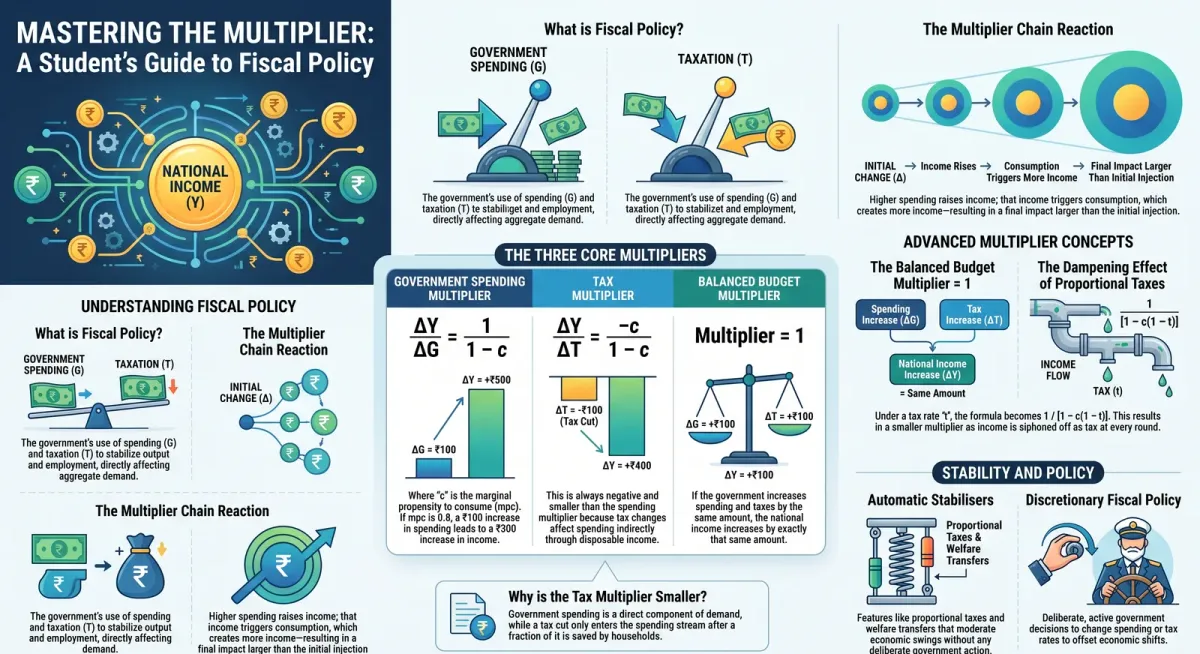
Fiscal policy refers to the government’s use of its spending and taxation powers to stabilise output and employment — an idea central to Keynes’s General Theory of Employment, Interest and Money. By adjusting government purchases (G) and taxes (T), the government directly affects aggregate demand and, through it, equilibrium national income.
The government affects equilibrium income in two ways: government purchases (G) add directly to aggregate demand, while taxes and transfers change the gap between income (Y) and disposable income (YD) available for consumption.
The Government Spending Multiplier
Government Spending Multiplier & Equilibrium Income Simulator
Adjust autonomous investment, autonomous consumption, and the Marginal Propensity to Consume (MPC) to observe changes in total equilibrium income and the multiplier effect.
Keynesian cross: equilibrium income
Equilibrium
At full employment
Planned spending equals full-employment output.
A positive planned-spending gap at Yf signals excess demand; the income gap and the spending gap are different quantities.
When government purchases rise, they add directly to aggregate spending. Because higher spending raises income, and higher income triggers further rounds of consumption spending, the final effect on equilibrium income exceeds the initial increase in G. This chain reaction is the multiplier effect.
Formula and Numerical Example
With lump-sum taxes, the government spending multiplier is:
ΔY / ΔG = 1 / (1 − c)
where c is the marginal propensity to consume (mpc).
Example: If mpc = 0.8, the multiplier = 1 / (1 − 0.8) = 1 / 0.2 = 5. So a ₹100 increase in government spending raises equilibrium income by ₹500.
The Tax Multiplier
A tax cut also boosts income, but through a different, weaker channel — it raises disposable income, which then raises consumption spending only by a fraction of the tax change.
ΔY / ΔT = −c / (1 − c)
Example: With mpc = 0.8, the tax multiplier = −0.8 / 0.2 = −4. A tax cut of ₹100 raises equilibrium income by ₹400 — smaller than the ₹500 increase from an equivalent rise in government spending.
Why It’s Smaller Than the Government Spending Multiplier
Government spending is itself a direct component of aggregate demand, so a rise in G enters the multiplier chain at full strength immediately. A tax change, by contrast, only affects spending indirectly — first it changes disposable income, and only a fraction c of that change actually gets spent. This is why, for any given mpc, the tax multiplier is always exactly one unit smaller in absolute value than the government spending multiplier.
The Balanced Budget Multiplier
What happens if government spending rises and taxes rise by the same amount, keeping the budget balanced? Adding the two multipliers together:
Balanced Budget Multiplier = 1/(1−c) + [−c/(1−c)] = (1−c)/(1−c) = 1
This means a ₹100 increase in both G and T (financed entirely by the tax increase) raises equilibrium income by exactly ₹100 — no more, no less. Intuitively, the full ₹100 rise in G triggers the full multiplier chain, while the ₹100 tax rise only dampens spending by a fraction (c) of itself at each round, so the two effects don’t fully cancel out — leaving a net gain equal to the size of the balanced increase.
Multiplier Under Proportional Taxes
The examples above assume lump-sum taxes — a fixed amount independent of income. In reality, most tax systems are proportional, where tax is a fixed fraction (t) of income: T = tY. This changes the multiplier to:
ΔY / ΔG = 1 / [1 − c(1 − t)]
Example: With mpc = 0.8 and a tax rate of t = 0.25, the multiplier = 1 / [1 − 0.8(0.75)] = 1 / [1 − 0.6] = 1 / 0.4 = 2.5 — noticeably smaller than the multiplier of 5 under lump-sum taxes.
This happens because proportional taxes reduce the effective marginal propensity to consume out of income to c(1−t): as income rises, part of it is automatically siphoned off as tax before it can be spent, muting the multiplier’s amplifying effect.
Automatic Stabilisers vs Discretionary Fiscal Policy
This dampening effect is actually useful — it’s why proportional income tax is called an automatic stabiliser. During a boom, rising incomes are partly absorbed by higher tax collections, restraining excessive consumption growth. During a slump, falling incomes mean lower tax liabilities, so disposable income and consumption fall by less than they otherwise would. Welfare transfers work similarly, rising during downturns to sustain consumption.
These stabilisers work automatically, without any government decision needed. Discretionary fiscal policy, by contrast, refers to deliberate changes in spending or taxes — for instance, raising G to offset a fall in private investment demand and keep autonomous expenditure, and therefore equilibrium income, unchanged.
Master Multiplier Numericals With Targeted Practice
Multiplier questions almost always appear as numericals in board exams — and the only way to build speed is by solving many variations. On ChampionsPrep , get AI-powered practice questions covering every multiplier formula in this chapter, built specifically for CBSE Class XII Commerce, at just ₹10 per use.
Test Your Knowledge

Government Spending Multiplier & Fiscal Policy Explained (Class 12)
Frequently Asked Questions
Why is the government spending multiplier always greater than 1? +
Because an initial increase in government spending triggers successive rounds of induced consumption spending (each household that receives the extra income spends a fraction of it, and so on), so the total effect on income exceeds the initial injection, as long as the marginal propensity to consume is between 0 and 1.
Is the tax multiplier positive or negative, and why? +
The tax multiplier is negative because an increase in taxes reduces disposable income, which reduces consumption and therefore reduces equilibrium income - taxes and income move in opposite directions.
What does a balanced budget multiplier of 1 actually mean? +
It means that if government spending and taxes rise by the same amount, equilibrium income rises by exactly that same amount - no more, even though the government spending multiplier alone is much larger than 1.
Why does a proportional tax reduce the size of the multiplier compared to a lump-sum tax? +
A proportional tax means that as income rises, a portion is automatically taxed away before it can be spent, lowering the effective marginal propensity to consume out of income and therefore weakening each successive round of the multiplier process.
What is the difference between an automatic stabiliser and discretionary fiscal policy? +
An automatic stabiliser (like proportional taxes or welfare transfers) works without any deliberate government decision, automatically moderating economic swings. Discretionary fiscal policy involves the government actively choosing to change spending or tax rates to stabilise the economy.
AI-powered practice — free to start