Aggregate Demand and Equilibrium Income in the Two-Sector Model | Class 12 Macroeconomics

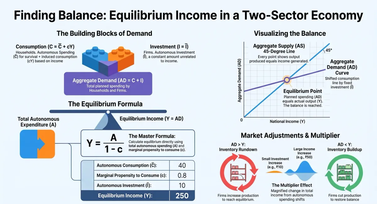
How does an economy decide how much total output to produce? In Class 12 Macroeconomics, the answer comes from the two-sector model, where equilibrium income is determined by the interaction of aggregate demand and aggregate supply. This is one of the highest-weightage topics in CBSE board exams and Commerce entrance tests, so let’s build it up step by step.

What Is Aggregate Demand in a Two-Sector Economy?

In an economy without a government, the two sources of final demand for goods and services are consumption (C) and investment (I). So, ex-ante aggregate demand is:

AD = C + I

We already know consumption follows the function C = C̄ + cY. For investment, this chapter makes a simplifying assumption: firms plan to invest the same amount every year, regardless of income. This gives us the ex-ante investment function:

I = Ī

where Ī is a positive constant representing autonomous investment. In reality, investment depends heavily on the market rate of interest and credit availability, but for now, we treat it as autonomous to keep the model simple.

Deriving the Aggregate Demand Equation

Substituting the consumption and investment functions into AD = C + I gives:

AD = C̄ + Ī + cY

If we combine the two autonomous terms, C̄ and Ī, into a single term A (total autonomous expenditure), the equation simplifies to:

AD = A + cY

It’s worth noting that C̄, representing subsistence consumption, tends to stay fairly stable over time, while Ī tends to fluctuate — a fact that becomes very important when we study business cycles later.

The Equilibrium Condition

The goods market is in equilibrium when planned (ex-ante) aggregate demand equals planned (ex-ante) aggregate supply, which is simply the level of output, Y:

Y = A + cY

Solving this for Y:

Y − cY = A

Y(1 − c) = A

Y = A / (1 − c)

This is the single most important formula in this chapter. It tells us the equilibrium level of income directly from the values of autonomous expenditure (A) and the marginal propensity to consume (c).

Worked Example

Suppose C = 40 + 0.8Y and I = 10. Then A = 40 + 10 = 50, and c = 0.8.

Y = 50 / (1 − 0.8) = 50 / 0.2 = 250

So the equilibrium level of income is ₹250 crore (or whatever unit the question specifies).

The Graphical Method: AD Curve and the 45° Line

Graphically, the AD curve is obtained by vertically adding the consumption function and the investment function — since AD = C + I at every level of income. Because investment is a constant, the AD curve is simply the consumption function shifted upward by the amount Ī, and it has the same slope as the consumption function (equal to c).

On the supply side, we draw a 45° line, which has the special property that every point on it has equal horizontal and vertical coordinates. This represents aggregate supply in the short run: whatever level of output the economy produces, that same amount is available for supply, since price levels are assumed fixed and unused resources allow output to expand smoothly.

Equilibrium occurs exactly where the AD curve intersects the 45° line. At any income level to the left of this point, AD exceeds output, causing inventories to run down and encouraging firms to produce more. At any point to the right, AD falls short of output, causing unintended inventory buildup and encouraging firms to cut production. Only at the intersection point is there no pressure for output to change.

What Happens When Aggregate Demand Changes?

Equilibrium income changes whenever aggregate demand changes. This can happen through:

1. A change in consumption — due to a change in autonomous consumption (C̄) or MPC (c)

2. A change in investment — due to changes in credit availability or the interest rate

For example, if investment rises from 10 to 20 in our worked example above, the new equilibrium becomes:

Y = (40 + 20) / (1 − 0.8) = 60 / 0.2 = 300

Notice that a ₹10 increase in investment led to a ₹50 increase in equilibrium income — five times the initial change. This “multiplied” effect is the investment multiplier, which the next topic in this chapter explores in detail.

Government in the Model (A Quick Note)

If a government is introduced, the equilibrium equation extends to:

Y = C̄ + Ī + G + c(Y − T)

Here, government expenditure (G) adds directly to aggregate demand, while taxes (T) reduce disposable income and therefore consumption. The term (G − cT) simply behaves like another autonomous term, without changing the underlying logic of the model.

Related Reading

• Consumption Function Explained: MPC, MPS, APC and APS for Class 12 Commerce

• Ex-Ante vs Ex-Post in Economics: Planned vs Actual Values Explained (Class 12)

Take Your Preparation Further

The two-sector equilibrium model appears in nearly every board exam paper, often combined with graph-based questions. Practising both the algebra and the diagrams together is the fastest way to build exam confidence.

👉 Explore ChampionsPrep for step-by-step solved numericals, AI-powered doubt resolution, and CBSE/board-aligned practice sets for Class 11 and 12 Commerce — at just ₹10 per use.

Test Your Knowledge

Q1.In a two-sector economy without a government, ex-ante aggregate demand is:

C + IC + I + GC + SI + S

Q2.With C = 40 + 0.8Y and I = 10, what is the equilibrium level of income?

200250300500

Q3.In that economy, investment rises from 10 to 20. What is the new equilibrium income?

260280300350

Q4.At an income level to the left of equilibrium, which statement is true?

Output exceeds AD, so inventories pile up unintentionallyAD equals output, so there is no pressure to changePlanned savings exceed planned investmentAD exceeds output, so inventories run down unexpectedly

Q5.The AD curve in this model has the same slope as the consumption function. This slope equals:

c, the MPC1s, the MPS1/(1 − c)